The Reachability Problem and Connections with Safety
We are now ready to look into the key part, i.e. how can we compute unsafe sets for an autonomous system and how can we design a safety-preserving controller?
There are many ways to compute these unsafe sets but we will primarily look into the Hamilton-Jacobi Reachability method to compute unsafe sets and safety-preserving controllers. The reason to study HJ reachability is its ability to seamlessly consider control bounds, uncertainty, or even state constraints while computing unsafe sets. Moreover, the reachability method is applicable to general nonlinear systems.
Let's start by looking into what the reachability problem is and then we will see how it is connected with the safety analysis of autonomous systems.
Reachability Problem
In reachability, we are interested in computing the Backward Reachable Tube (BRT) of a dynamic system. BRT is the set of all starting states of the system that will eventually reach some target set despite the best control effort.
If the target set represents the failure set of a system then BRT represents the potential unsafe set of states for the system and thus should be avoided. Pictorially:
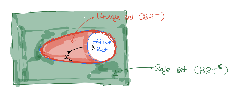
Conversely, the complement of BRT represents the set of safe states for the system.
Mathematically, let
L⊆Rn be the target set (typically failure set)
BRT(t)⊆Rn be the BRT at time t (typically unsafe set)
BRT(t)={x:∀u(⋅)∈UtT,∃d(⋅)∈DtT,ξx,tu,d(s)∈L for some s∈[t,T]}
Intuitively, BRT(t) computes the set of all starting states from which no matter what control does, there exists a disturbance, that will drive the system inside the target set (or the failure set).
In other words, to compute the unsafe set we need to compute the BRT of the failure set.
Examples of the Failure Sets
A high turbulence region for an aircraft.
Ceiling, floor for an indoor autonomous drone.
A no-go zone for a warehouse robot.
An unmapped area for an autonomous car.
Example
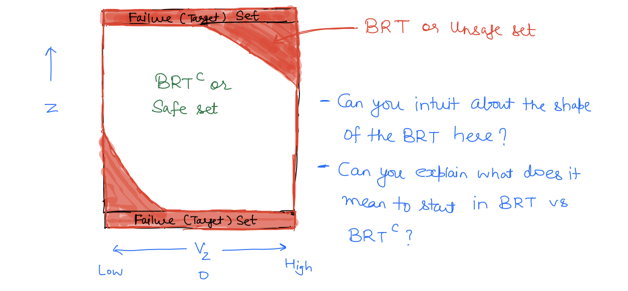
Let's go back to our 2D drone example where the drone is moving up and down inside a room.
Here, the failure set is given by the ceiling and the floor. As we will see later, the BRT is given as follows:
Hamilton-Jacobi Reachability
Now that we have established a connection between the BRT and the unsafe set of a system, let's talk about how we can compute the BRT. Once again, there are many methods proposed to compute the BRT; we will particularly look into HJ reachability that formulates the BRT computation as an optimal control problem. This allows us to use all the optimal control tools that we have learned so far to compute the BRT.
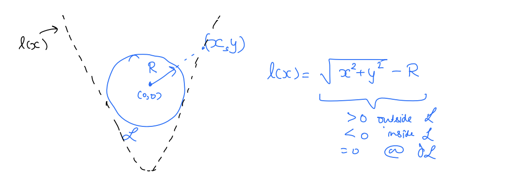
Specifically, HJ reachability leverages level set methods to convert the BRT computation into an optimal control problem. First, we define a target function l(x) to implicitly represent the target set L, i.e., L={x:l(x)≤0}. In other words,
l(x)≤0⇔x∈L Thus, the target set is given by the subzero level of the target function l(x).
- One such function is signed distance to L.
- Signed-distance >0 when x is outside L
- Signed-distance <0 when x is inside L
- Signed-distance =0 when x is at the boundary of L
- As an example, imagine the target set is a circle of radius R centered at the origin.
Converting to an OC Problem
Recall that we are formulating BRT computation as an optimal control problem. For an optimal control problem, we need a cost function. To do so, we define the following cost function:
J(x,u(⋅),d(⋅),t)=s∈[tsT]minl(x(s)) J represents the minimum signed distance achieved by the trajectory starting at x during the time horizon [t,T] under the control u(⋅) and disturbance d(⋅). Let's understand this cost function a bit better.
Case 1:
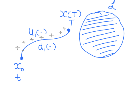
J(x0,u1(⋅),d1(⋅),t)>0 Case 2:
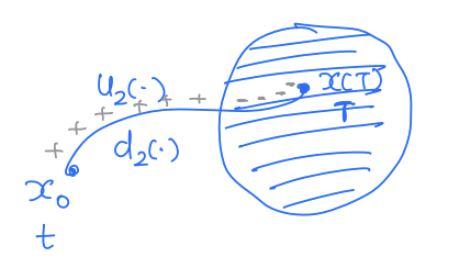
J(x0,u2(⋅),d2(⋅),t)<0 Case 3:
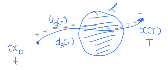
J(x0,u3(⋅),d3(⋅),t)<0
Thus, by looking at the sign of J, we can tell whether the trajectory ever entered the target set or not under a given control and disturbance function. If we want to keep the system safe, the control should try to keep the system outside the target set as much as it can, i.e., it should try to maximize J and the disturbance should try to minimize J. Thus, our optimal control problem reads:
V(x,t)=u(⋅)∈Γumaxd(⋅)∈ΓdminJ(x,u(⋅),d(⋅),t)=u(⋅)∈Γumaxd(⋅)∈Γdmin(s∈[t,T]minl(x(s))) Now suppose that V(x0,t)<0 for some state x0. This means that the control tried but couldn't do anything to avoid getting the system into the target set. In other words, x0∈BRT(t).
Similarly, if V(x0,t)>0. This means that the control was successful in keeping the system trajectory outside the target set despite the worst-case uncertainty. In other words, x0∈/BRT(t).
Thus, once we have the value function, we can compute the BRT as:
BRT(t)={x:V(x,t)≤0} Solving the OC Problem
Great! We now have an optimal control problem whose solution can give us the BRT. So all that remains is to solve the optimal control problem. The issue is that the cost function of this OC problem is different -- it is no longer a running cost as we had earlier, rather it is a minimum operation over time. The good news is that we can still use the principle of optimality and dynamic programming to compute the value function.
Recall that,
V(x,t)=u(⋅)maxd(⋅)mins∈[t,T]minl(x(s))=u(⋅)maxd(⋅)minmin{s∈[t,t+δ]minl(x(s)),z∈[t+δ,T]minl(x(z))}=u(⋅)maxd(⋅)minmin{s∈[t,t+δ]minl(x(s)),J(x(t+δ),u(⋅),d(⋅),t+δ)}=u(⋅)maxd(⋅)minmin{s∈[t,t+δ]minl(x(s)),V(x(t+δ),t+δ)}=u(⋅)maxd(⋅)minmin{l(x),V(x(t+δ),t+δ)} As before, we will do the Taylor expansion of V(x(t+δ),t+δ)
V(x(t+δ),t+δ)≈V(x,t)+∂x∂V⋅dx+∂t∂V⋅δ+ h.o.t. ≈V(x,t)+∂x∂V⋅f(x,u,d)δ+∂t∂V⋅δ Thus, we have:
V(x,t)=u(⋅)mind(⋅)maxmin{l(x),V(x,t)+∂x∂V⋅f(x,u,d)δ+∂t∂Vδ}=u(t)mind(t)maxmin{l(x),V(x,t)+∂x∂V⋅f(x,u,d)δ+∂t∂Vδ}=min{l(x),V(x,t)+∂t∂Vδ+umindmax∂x∂V⋅f(x,u,d)δ}⇒min{l(x)−V(x,t),δ(∂t∂V+umindmax∂x∂V⋅f(x,u,d))}=0 Since this statement is true for all δ>0, we have:
≡min{l(x)−V(x,t),∂t∂V+umindmax∂x∂V⋅f(x,u,d)}=0min{∂t∂V+umindmax∂x∂V⋅f(x,u,d),l(x)−V(x,t)}=0 This is called HJI Variational Inequality (HJI-VI). HJI-VI is very similar to HJI PDE with an additional term of l(x)−V(x,t). But as we will see next, the set of tools for solving HJI PDE can also be used to solve HJI-VI.